Decision Tree algorithm with example.
Basic algorithm (greedy algorithm)
Tree is constructed in a top-down recursive divide-and-conquer manner.
At start, all the training examples are at the root.
Attributes are categorical (if continuous-valued, they are discretized in advance).
Examples are partitioned recursively based on selected attributes.
Test attributes are selected on the basis of a heuristic or statistical measure (e.g., information gain).
When all samples for a given node belong to a same class, or no remaining attributes for further partitioning, or no more samples left, partitioning end.
Information Gain (ID3/C4.5)
Information Gain is a attribute selection measure.
The basic idea is to select the attribute with the highest information gain.
D as a data partition
Expected information
(entropy) needed to classify a tuple in D
Information
needed (after using A to split D into v partitions) to classify D
Information gained
by branching on attribute A
Example
if we have a database below and want to build a decision tree for “who will buy the computer”
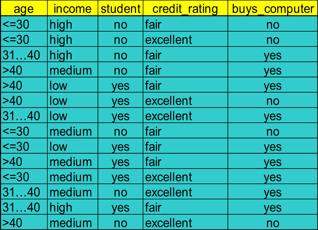
Class N: buys_computer = “yes”
Class M: buys_computer = “no”
First, select a attribute to calculate the Gain. Here we choose age.
| Age | |||
|---|---|---|---|
| <= 30 | 2 | 3 | 0.971 |
| 31-40 | 4 | 0 | 0 |
| > 40 | 3 | 2 | 0.971 |
| 9 | 5 | 0.940 |
Similarly, we have to calculate Gains of other attributes:
Gain(income) = 0.029
Gain(student) = 0.151
Gain(credit, rating) = 0.048
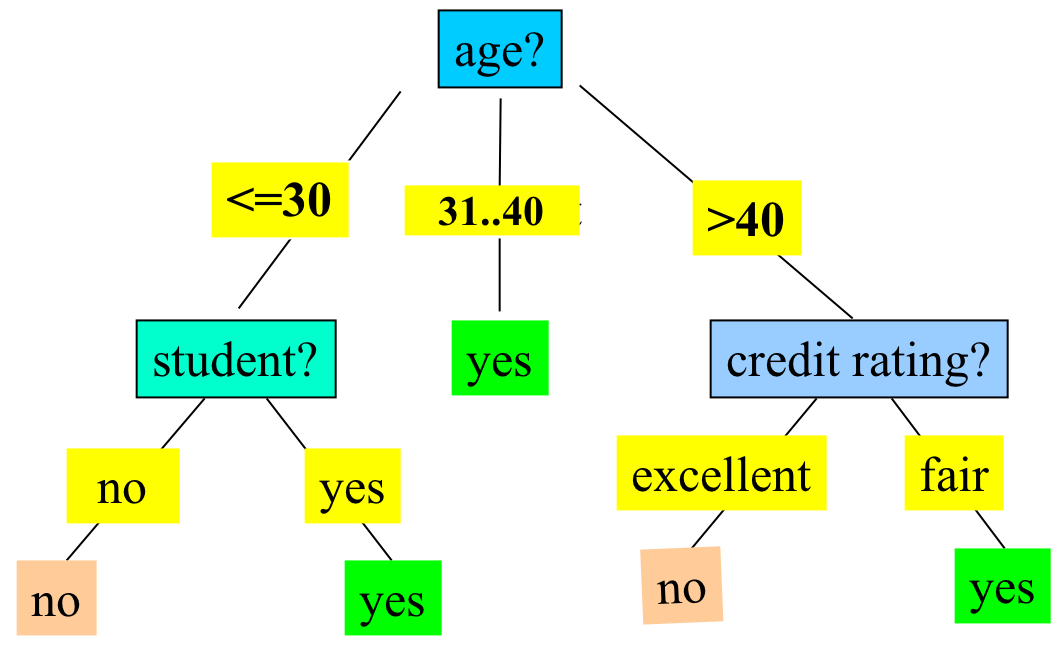
Finally we get a decision tree below.
Gain Ratio (C4.5)
Gain is another attribute selection measure
Information gain measure is biased towards attributes with a large number of values. C4.5 (a successor of ID3) uses gain ratio to overcome the problem (normalization to information gain)
For example:
The attribute with the maximum gain ratio is selected as the splitting attribute.
Gini index (CART, IBM IntelligentMiner)
If a data set D contains examples from n classes, and the is the relative frequency of class j in D, the gini index, gini(D) is defined as
If a data set D is split on A into two subsets D1 and D2, the gini index is defined as
Reduction in impurity:
The attribute that has the lowest (or the greatest reduction in impurity) is chosen to split the node (need to enumerate all the possible splitting points for each attribute)
In the example above, D Has 9 tuples in buy_computer = “yes” and 5 in “no”
Suppose the attribute income partitions D into D1: {low, medium} = 10 and D2: {high} = 4
However, =0,30 ,which is the lowest thus the best.
All attributes are assumed continuous-valued
Sometimes we may need other tools, e.g., clustering, to get the possible split values
Can be modified for categorical attributes
Comparison
Information gain: Bias toward multivalued attributes.
Gain ratio: Tends to prefer unbalanced splits in which one partition is much smaller than the others
Gini index:
- Bias toward multivalued attributes.
- Hard to deal with the dataset that has large number of classes.
- Tends to favor tests that result in equal-sized partitions and purity in both partitions
Reference
Han, J., Kamber, M., & Pei, J. (2011). Data Mining: Concepts and Techniques (3rd ed.). Burlington: Elsevier Science.